Home
Tutorial: Pair distance distribution, p(r)
Tutorial contributors: Andreas Haahr Larsen
Learning outcomes
- Be able to generate the pair distance distribution, p(r), from a SAXS or SANS dataset.
- Recognize geometrical objects from their p(r).
- Mention circumstances can lead to a negative p(r).
- Detect aggregation from the shape of the p(r).
Introductory remarks
SAS data is measured in "reciprocal space", i.e. as function of 1/length. By a Fourier transformation, one can get a distribution of distances between scattering pairs in the sample (weighted by contrast): the pair distance distribuion or simply the "p(r)" (colloquially denoted the "p-of-r-function").
The p(r) is in "real space", i.e. as function of length, so it can be interpreted more intuitively than the data itself. The p(r) provides useful structural information about the sample prior to any modelling.
This is a practical tutorial, but if you wish to get a better understanding of the theory, it is recommended that you work with the exercises at pan-learning.org, covering some simple examples.
SAXS or SANS data can generally not be Fourier transformed directly for the following reasons: (1) Data is measured in a limited range and not from minus infinity to plus infinity (2) Data is noisy. Therefore, the p(r) is generated by an Indirect Fourier transformation (IFT) .
Various IFT algorithms are implemented and can be accessed through different software packages. In this tutorial, we will use BayesApp.
Part 1: Recognizing shapes from the pair distribution, p(r)
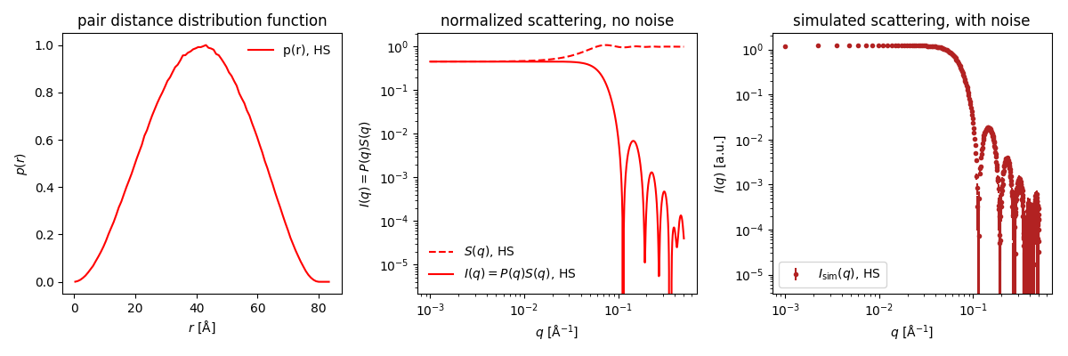
Go to: Shape2SAS, and simulate a sphere with radius of 50 Å as Model 1 and a 30 Å sphere as Model 2.
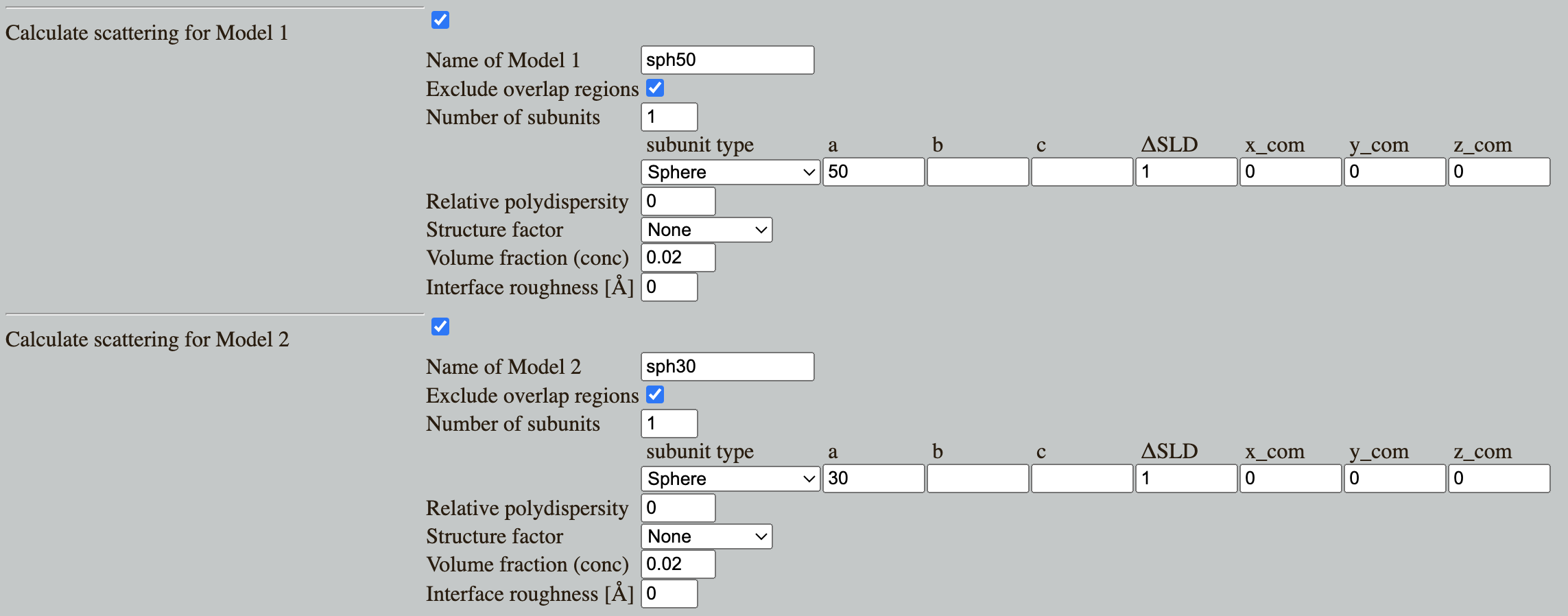
Shape2SAS plots the p(r) (lef), the normalized scattering (middle panel) and simulated data (right panel):
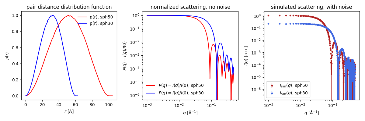
Can you guess from the shapes of the p(r) functions which one represents the larger which one represents the smaller spheres?.
For homogeneous particles (i.e., having the same contrast in the whole particle), p(r) is the probability distribution of distances between pairs of scatterers in the particle. What is the most frequent distance? What is the largest distance? The largest distance is denoted the dmax.
Try to guess how the p(r) look for an ellipsoid and or for a cylinder or an a hollow sphere. Calculate the p(r) for these and other shapes using Shape2SAS.
Part 2: Calculating the pair distribution, p(r), from SAXS/SANS data
Download the simulated data of the sphere with radius of 50 Å, which you generated with Shape2SAS, or use this example data.
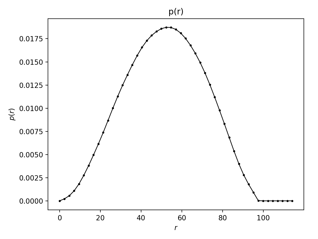
Go to BayesApp, which is a web-application for generating p(r) for SAXS and SANS data.
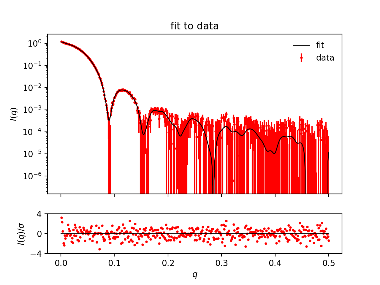
Upload your simulated data, and press submit.
The program shows the calculated p(r), and a fit to the data, which was used to generate this p(r).
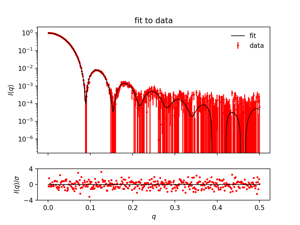
Give a rough estimate of the maximum distance (this does not have to be accurate) and press submit again. Giving an estimate of the maximum distance is optional, but makes BayesApp faster and more robust. Notice the computation time decreased.
Go to the SAS biological data bank (SASBDB), which is a database for SAXS and SANS data. Download the SAXS data of the protein Xylanase (SASBDB entry: SASDPS4): SASDPS4.dat.
Use BayesApp to calculate the p(r). To increase speed and robustness, provide a rough estimate of the maximum distance - it does not have to be precise.
Comment on the resulting p(r). Notice that the p(r) looks like the p(r) from a sphere, meaning the protein is globular (approximately spherical). See the actual shape of the protein in the SASBDB entry.
Now, do the same for an elongated protein, SASBDB entry: SASDTE2.
Notice how the p(r) is closer to that of a cylinder or elongated ellipsoid. This way, by looking at the p(r), one can get an idea of the shape of the particles without model fitting.
Part 3: Inhomogeneous particles
The p(r) is a contrast-weighted pair distribution (contrast = ΔSLD = excess scattering length density). I.e. each bin in the distribution is the weighted sum of all pairs with a given distance.
Therefore, if a pair of scatterers have contrasts with the same sign, then they contribute positively, but if the signs are opposite, then their contribution to the p(r) is negative. This means that the p(r) can have negative values.
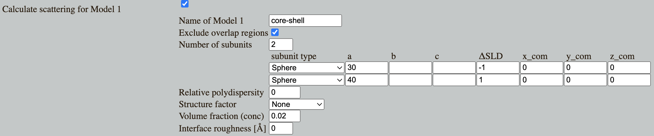
Go to Shape2SAS, and simulate a core-shell spherical particle with inner radius 30 Å and outer radius 40 Å and with core ΔSLD of -1 and shell ΔSLD of +1
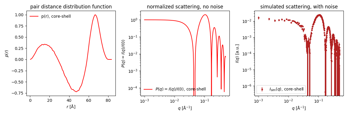
- Negative contribution comes from scattering pairs with ΔSLDs having opposite signs. Likewise, positive contributions comes from pair having the same sign (either both positive or both negative ΔSLD). Using this information, consider:
- What scattering pairs in the core-shell particle does the negative part of the p(r) represent?
- Why are pair distributions (including this one) positive as small values of r?
- Why is this p(r) positive at larger r?
Download the simulated data (example data) and upload it to BayesApp. Give an estimate of the maximum distance and press Submit.
By default, the p(r) is constraint to be positive. (Transformation: Debye). Now, try to rerun with Tranform: Negative (i.e. p(r) can be negative.) Is the result better?
Compare with the true p(r), which was simulated in Shape2SAS.
Note that inhomogeneous particles do not always give rise to p(r) with negative contribution. Try, for example, simulating a core-shell spherical particle with core radius of 20 and ΔSLD of -1 and shell radius of 40 and ΔSLD of +1.
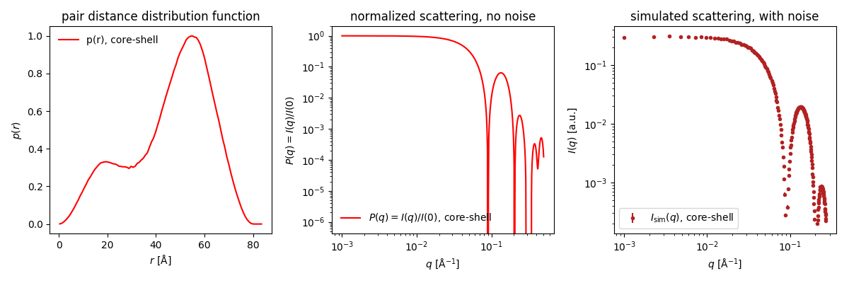
In this case, the negative contribution from core-shell scatterer pairs is cancelled out by positive contributions from shell-shell scatterer pairs having the same distance.
Part 4: Interparticle interactions
Negative contribution in the p(r) may also stem from interparticle interactions. This can appear if the concentration is high.
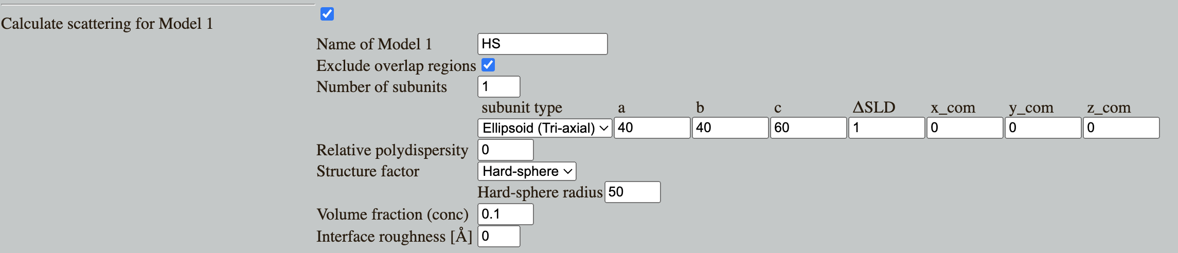
Go to Shape2SAS, and simulate an ellipsoid with axes 40,40 and 60 Å. Add interparticle interaction, modelled with a hard-sphere structure factor with hard sphere radius of 50 and volume fraction 0.1.
The p(r) in Shape2SAS is calculated before the structure factor.
Download thedata data and generate the p(r) using BayesApp. Try with positive restraint (Transformation: Debye) or without (Transformation: Negative).
Part 5: Protein aggregation
Protein aggregation in a sample may be detected using p(r) - in reveals itself as a "tail" towards high values of r. In this case, the p(r) can be considered a linear combination of the p(r) of a non-agregated particle with a small dmax, and the p(r) of an aggregate with a large dmax.
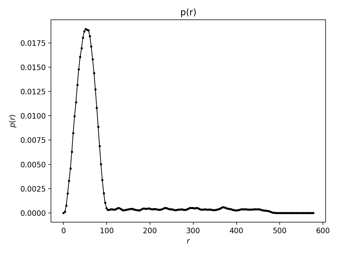
Go to Shape2SAS, and simulate a 50 Å sphere (or any other object) with aggregate structure factor (set fraction to 0.005, i.e. 0.5% of all particles are aggregated and particles per aggregate to 40).
OBS: The p(r) shown in Shape2SAS is for the spheres without the structure factor, but the simulated data contains the structure factor.
Download the data (example data), and calculate the p(r) with BayesApp. (The default number of points in p(r) may need to be increased). Notice the "tail":
Challenges
- The protein bovine serum albumin (BSA) was measured with SAXS. Data: bsa_hc_030.dat. BSA is a common blood protein. The sample was measure with SAXS at relatively high concentration. Generate the p(r) - what does it tell you?
- A sample of discoidal particles (diameter ca 5 nm, as estimated from negative stain electron microscopy) was measured in SAXS at neutral pH (neutral pH data) and pH 5.0 (low pH data). Using the p(r), describe what happens?
- The protein GluA2 (glutamine receptor - important for neuronal communication) was measured with SANS. Data: SASDD26.dat. You have calculated the theoretical dmax to be around 200 Å. From the p(r), what can you tell about the sample?
Feedback
You can help us improve the tutorials by filling out this short feedback form (it takes 2 min).
Home
Frontpage image from Larsen 2018 (PhD Thesis)