Home
Tutotial: Spheres
Tutorial contributors: Andreas Haahr Larsen, Martin Cramer Pedersen, Jacob Kirkensgaard, Viktor Holm-Janas.
Before you start
- Download and install SasView (on MacOS: you need to install Xcode first)
Learning outcomes
- Simulate SAS data of spherical particles, and determine which sample contains the larger particles, by visually comparing the curves.
- Describe the difference between the scattering from spheres and ellipsoids.
- Recognize interparticle interaction in a small-angle scattering experiment and know under what conditions this may happen.
- Descriminate a sample of polydisperse spheres from a sample of monodisperse spheres.
- Be able to fit a sphere in SasView and determine its size, and size distribution if it is polydisperse.
- Using the above, be able to analyze structural changes in samples, based on SAS data measured at different conditions.
Part 1: Monodisperse spheres
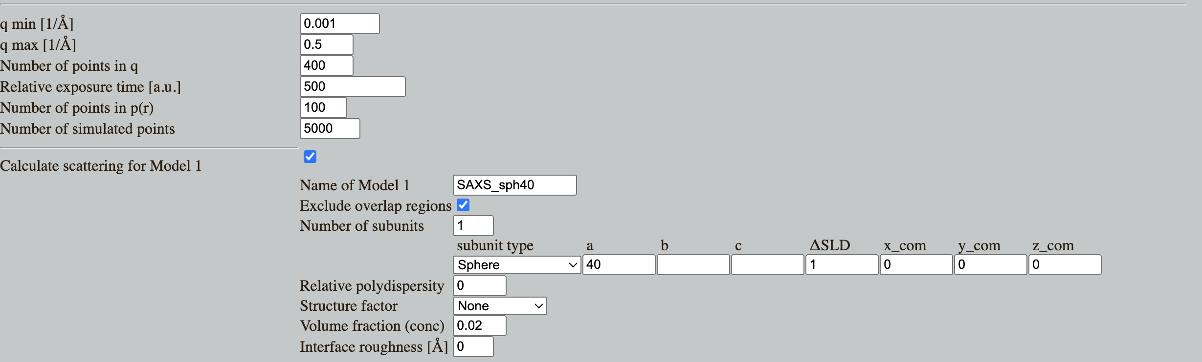
Go to: Shape2SAS, and simulate a sphere with a 40 Å radius. You may have to click on the three lines in the top-left of the window, then "Calculations". Set parameters.
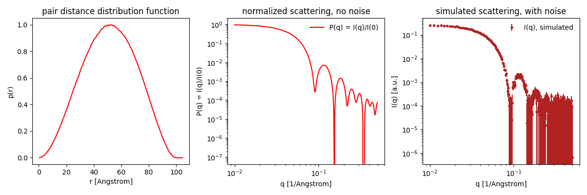
- Press Submit. Shape2SAS generates three plots (besides from visualization of the particle):
- A pair distance distribution. This is a useful tool in SAXS and SANS analysis, but will not be used in this tutorial. See the tutorial: Pair distance distribution, p(r).
- Calculated scattering, normalized. This is the form factor, P(q). It contains information about the size and shape of the particle.
- Simulated scattering, showing what real SAXS or SANS data for that sample may look like, if actually measured.
Comment on the resulting scattering. Try to compare with a smaller or larger sphere (as Model 2), and with other shapes. Notice the inverse relation: larger particles have features at smaller q.
Download the data you just simulated: Isim.dat (or use this example data) (right click - save as...).
- Load the data into SasView and fit with an analytical sphere model:
- Press "Load data" and select the data you simulated. Normally you would here choose experimentally measured SAXS or SANS data.
- "Send data to" and choose "Fitting" in the drop-down menu.
- Your data should appear in the Fit panel (a separate window).
- Choose model category "sphere" from the first drop-down menu. There are many different sphere-like models, choose "sphere" under model name (second drop-down menu).
- Now you have some model parameters. You can click/select those you want to fit.
- Compute/plot give you the model scattering with the default values - this shows data (blue) and model (orange) together. The residuals plot (difference between model and data) is also shown.
- You can try to adjust some parameters manually, and pres compute again. Try to manually find some resonable values for scaling, background and radius.
- Try changing the value of the radius to see what happens - notice the inverse relation: larger radius moves all the features to smaller q values.
- Try to fit: check the boxes: scale, background and radius, and press "Fit".
- A convergence plot is shown along with the previous windows - this just shows that the fitting algoritm has converged, and you can ignore that.
Shown below is an example of a fit to samples of 50 Å spheres - how does it compare to your results?:
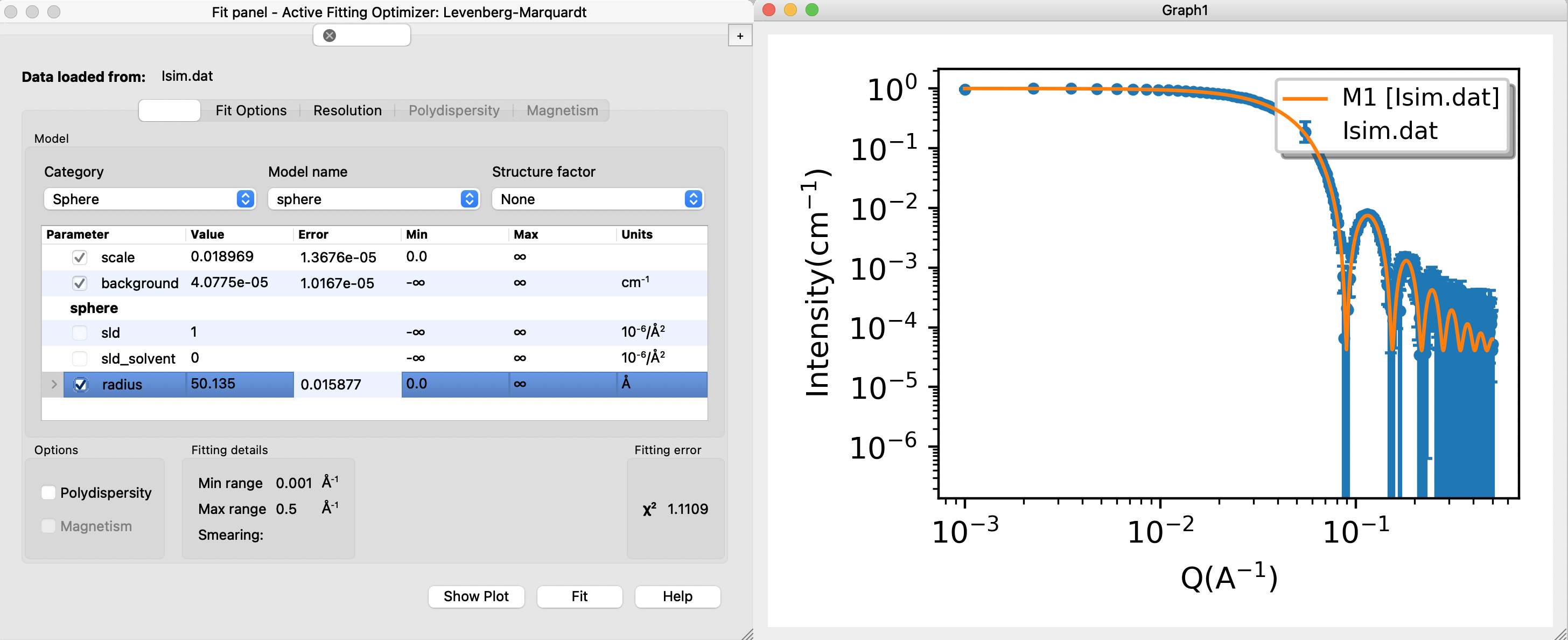
Does the fitted radius match the input for your simulations (40 Å)? Is the fit "good" - as assesed by visual inspection and the reduced χ 2. This value is displayed in the Fit panel.
Try doing the same for elipsoids. In SasView, these can be modelled with an ellipsoid of revolution (two radii are the same, one different), or a tri-axial ellipsoid (all radii are different). Note: for the ellipsoid of revolution model in SasView, ensure that you to use the right values for R_e (the two identical radii) and R_p (the other radius).
Try also to simulate and fit a cylinder.
Part 2: Polydisperse spheres
Polydispersity means that there are particles with different shapes or sizes in the sample, following some size distribution. That could be spherical nanoparticles with some variation in their radius.
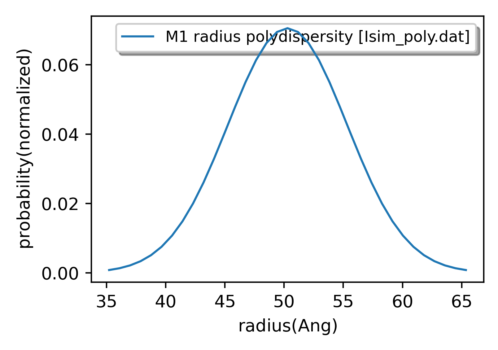
Go to: Shape2SAS, and simulate a sphere with a radius of 50 Å as Model 1 (monodisperse sample) and a sphere with radius of 50 Å and relative polydispersity of 0.1 as Model 2 (polydisperse sample).
The simulated data may look like this:
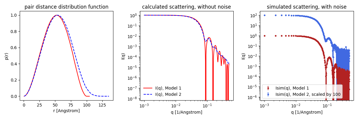
Comment on the results. Why is the features "smeared out" in the polydisperse sample? Try to vary the degree of polydispersity.
Try also to compare the scattering from polydisperse spheres with that of ellipsoid with semiaxes a = 50 Å, b = 40 Å, c = 60 Å.
Note: a Gaussian (normal) size distribution is used to simulate polydispersity in Shape2SAS, but many different size distributions are possible in real samples (Pauw et al 2013).
Load your data (or you can use this example data) into SasView and model the polydispersity. You need some extra steps, besides those you did in Part I:
- load the data as before, and choose the sphere model. Try to fit the data with a monodisperse model as good as possible.
- to include polydispersity, click the "Polydispersity" option in the lower left corner of the Fit panel.
- click the (now active) "polydispersity" tab in the Fit Panel. check the box "Distribution of radius". Give a non-zero number as default for PD (stands for polydispersity).
- on the right side, it says that it is assuming a Gaussian distribution (a normal distribution). This is fine, but other distributions can be chosen.
- press fit
- besides from fit, residuals and convergence, you also get a window with the fitted distibution of radii of spheres in the sample. By default it plots on log-log. If you right-click, choose change scale to x and y (instead of logarithmic), you will recognise that the a normal distribution in the radius.
Part 3: Spheres with interparticle repulsion (hard-sphere structure factor)
If the concentration of particles in as sample is high, they may frequently "bump into each other". This will give rise to some characteristic distances (2 times the radius), which gives rise to change of the scattering.
The additional scattering can (for some samples) be described by a so-called hard-sphere structure factor.
Go to: Shape2SAS, and simulate a sphere with a radius of 50 Å as Model 1 and a sphere with radius of 50 Å and hard sphere structure factor with volume fraction 0.2 and hard-sphere interaction radius of 50 Å as Model 2.
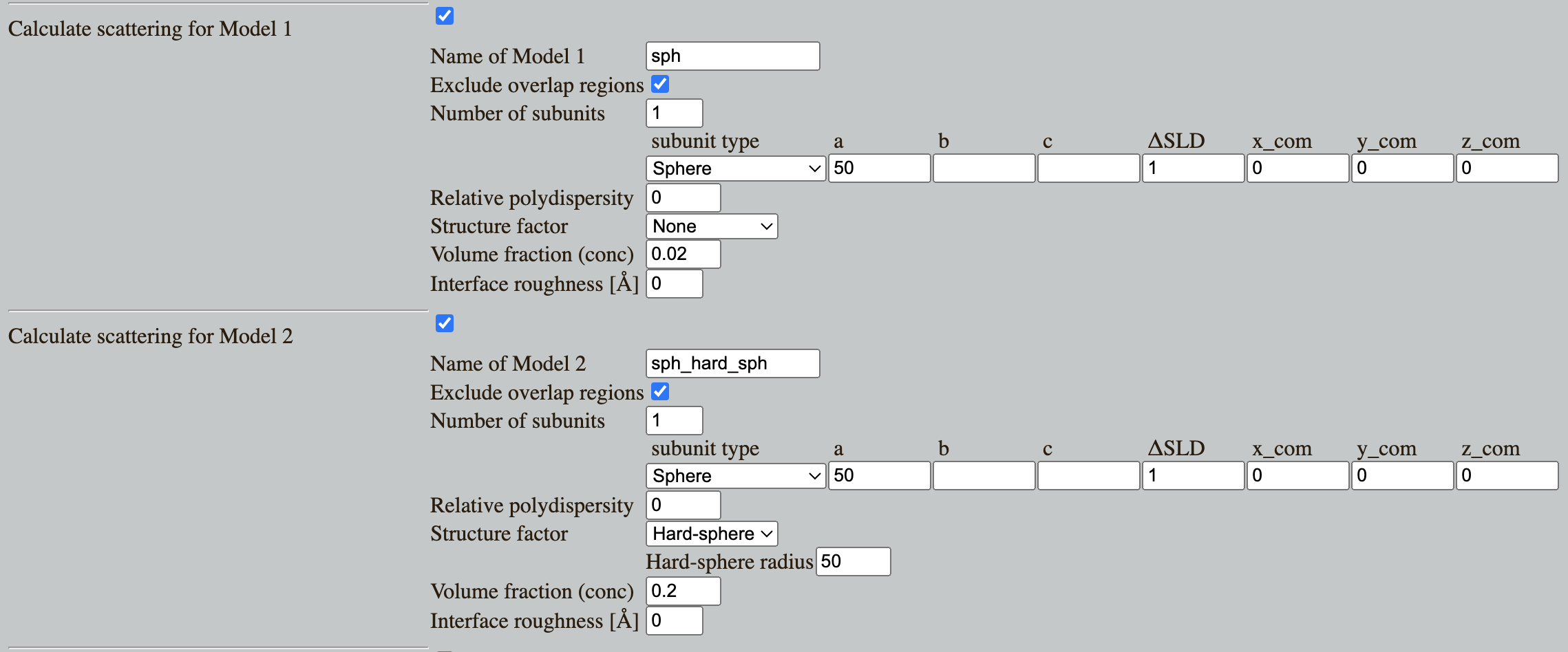
Comment on the results. You will notice a "dip" at low-q, which is characteristic. If an experimentalist is not interested in this effect, it may be removed by lowering the sample concentration. You may try to decrease the volume fraction in the simulations (i.e the concentration), to see the structure factor effect disappear.
- Fit the data is SasView:
- Download the simulated data for Model 2 (with hard-sphere structure factor and volume fraction 0.2) (or use this example data)
- Load the data into SasView and fit a sphere form factor like before (no polydispersity) - observe how the model fit deviates from the data
- Add a hard-sphere structure factor to the fit. Structure factors are selected in the third drop-down menu in the Fit panel.
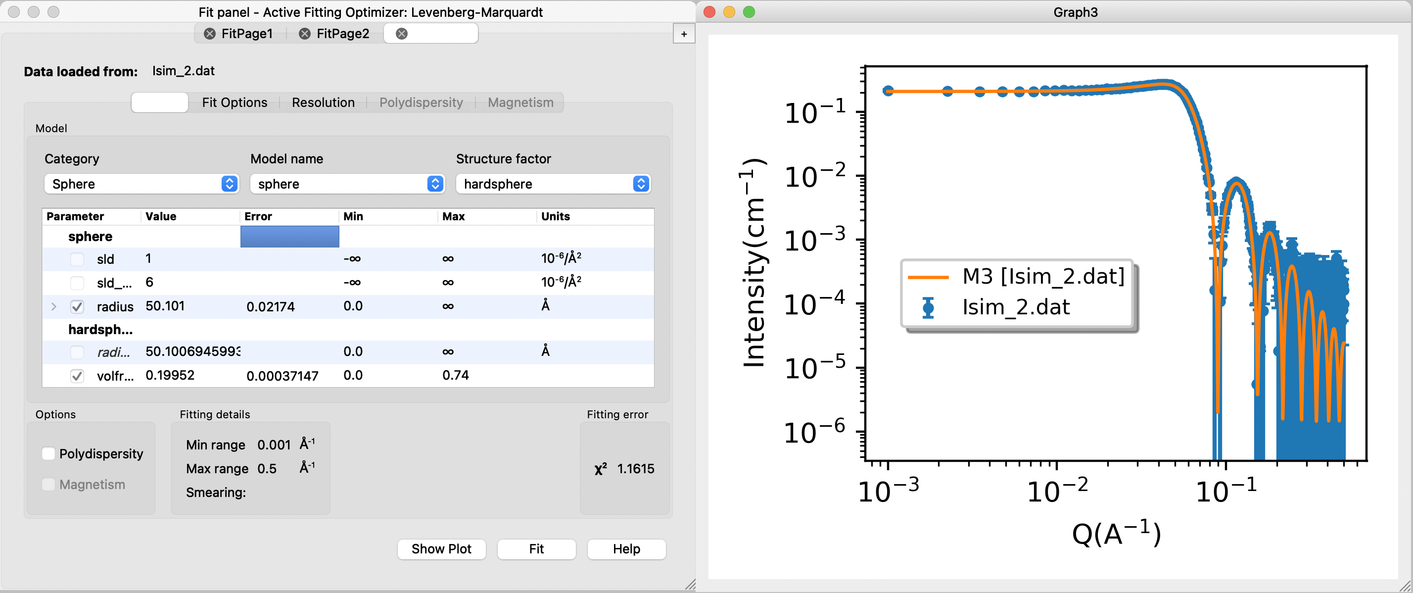
Does the fitted values match the input values for the simulations?
Part 4: Spheres with a fraction of aggregated spheres (fractal structure factor)
Some particles have a tendency to aggregate (be "sticky"). This may be proteins or nanoparticles. If a part of the sample aggregates, the scattering will be a sum of the scattering from the aggregate and that from the non-aggregated particles.
Aggregates may also be described by a structure factor (although very different from the hard-sphere structure facotor), and as we shall see, having the opposite effect.
Go to: Shape2SAS, and simulate a sphere with a radius of 50 Å as Model 1 and a sphere with radius of 50 Å and aggregate structure factor with fraction of 0.01 (i.e. 1% of the particles are in an aggregate), effective radius of 50 Å, and 80 particles per aggregate as Model 2.
Model 1 corresponds to a sample without aggregation, and Model 2 corresponds to a sample, where 1% of the spheres are in aggregated form, with 80 spheres per aggregate. The resulting scattering may look like this (note: the aggregation is not included in the p(r)):

Comment the results. Try varying the fraction (i.e., degree of aggregation) and the number of particles per aggregate (the size of the aggregates). Notice how this results in an upturn at low-q - i.e. opposite the dip at low-q for the hard-sphere structure factor.
Note on the aggregate model: a 2-dimensional fractal aggregate structure factor (Larsen, Pedersen and Arleth 2020) was used to simulate aggregation in Shape2SAS, but many different aggregates are possible in a real sample.
Currently, this structure factor is not implemented in SasView - maybe this is a task for you?
Challenges
- Spherical nanoparticles were measured at high concentration (high conc data) and low concentration (low conc data). What are their shape and size (distribution)?
Tip: to compare data in sasview, Load data, select the data and under plot press "Create new" - A sample of discoidal particles (diameter ca 5 nm, as estimated from negative stain electron microscopy) was measured in SAXS at neutral pH (neutral pH data) and pH 5.0 (low pH data). What happens?
Feedback
By filling this feedback form you can help us improve the tutorials (it takes 2 min).